Using CellHint for cell type harmonisation

This notebook showcases how to perform cross-dataset cell type harmonisation using CellHint.

Only the main steps and key parameters are introduced in this notebook. Refer to detailed Usage if you want to learn more.

We try to answer three questions:

• Different labs annotate cell types differently (naming convention, annotation resolution, etc.) - how to unify these cell types into a common framework?

• Transcriptome-based hierarchical clustering of cell types does not necessarily mirror biological lineages - how to integrate knowledge across studies to reflect cell type hierarchies?

• Cells are usually annotated only by the dataset of origin - how to re-annotate these cells within the context of multiple studies?

Download and process four spleen datasets

import scanpy as sc

adata = sc.read('cellhint_demo_folder/Spleen.h5ad', backup_url = 'https://celltypist.cog.sanger.ac.uk/Resources/Organ_atlas/Spleen/Spleen.h5ad')
adata

AnnData object with n_obs × n_vars = 200664 × 74369
    obs: 'Dataset', 'donor_id', 'development_stage', 'sex', 'suspension_type', 'assay', 'Original_annotation', 'CellTypist_harmonised_group', 'cell_type', 'Curated_annotation'
    var: 'exist_in_Madissoon2020', 'exist_in_Tabula2022', 'exist_in_DominguezConde2022', 'exist_in_He2020'
    uns: 'schema_version', 'title'
    obsm: 'X_umap'

This dataset combines cells from four studies, and is one of the organ atlases in CellTypist.

adata.obs.Dataset.value_counts()

Madissoon et al. 2020          92049
Dominguez Conde et al. 2022    70099
Tabula Sapiens 2022            34004
He et al. 2020                  4512
Name: Dataset, dtype: int64

Log-normalised gene expression (to 10,000 counts per cell) is in .X, and raw counts are in .raw. CellHint does not rely on the latter, but here we still start from raw counts for completeness of a single-cell pipeline.

adata = adata.raw.to_adata()

Delete everything in the adata except .X and .obs for clarity of this tutorial.

del adata.var
del adata.uns
del adata.obsm
adata

AnnData object with n_obs × n_vars = 200664 × 74369
    obs: 'Dataset', 'donor_id', 'development_stage', 'sex', 'suspension_type', 'assay', 'Original_annotation', 'CellTypist_harmonised_group', 'cell_type', 'Curated_annotation'

Perform a canonical single-cell workflow from normalisation, highly variable genes (HVGs) identification, scaling, PCA, neighborhood construction to low-dimensional visualisation.

sc.pp.normalize_total(adata, target_sum = 1e4)
sc.pp.log1p(adata)
sc.pp.highly_variable_genes(adata, batch_key = 'Dataset', subset = True)
sc.pp.scale(adata, max_value = 10)
sc.tl.pca(adata)
sc.pp.neighbors(adata)
sc.tl.umap(adata)

/opt/conda/lib/python3.8/site-packages/pandas/core/arrays/categorical.py:2487: FutureWarning: The `inplace` parameter in pandas.Categorical.remove_unused_categories is deprecated and will be removed in a future version.
  res = method(*args, **kwargs)
/opt/conda/lib/python3.8/site-packages/pandas/core/arrays/categorical.py:2487: FutureWarning: The `inplace` parameter in pandas.Categorical.remove_unused_categories is deprecated and will be removed in a future version.
  res = method(*args, **kwargs)

N.B.: Selection of HVGs is important for most single-cell tasks. Please find out the HVGs most suiting your data.

Visualise the dataset of origin (Dataset) and original author annotations (Original_annotation).

sc.pl.umap(adata, color = 'Dataset')

sc.pl.umap(adata, color = 'Original_annotation')

As expected, strong batches exist; meanwhile, cell types are annotated differently across studies (by different authors).

Perform cell type harmonisation

The input AnnData needs two columns in .obs representing dataset origin and cell original annotation, respectively. We will use the function cellhint.harmonize to harmonise cell types across datasets.

import cellhint

alignment = cellhint.harmonize(adata, 'Dataset', 'Original_annotation')

👀 Detected PCA coordinates in the object, will use these to calculate distances
🏆 Reordering datasets
🖇 Harmonizing cell types of Dominguez Conde et al. 2022 and Madissoon et al. 2020
🖇 Harmonizing cell types of Tabula Sapiens 2022
🖇 Harmonizing cell types of He et al. 2020
🖋️ Reannotating cells
✅ Harmonization done!

By default, PCA (X_pca) is used as the search space, which is noisy as the batch effect is not corrected. However, this is usually not a problem for cellhint.harmonize due to an internal normalisation procedure applied. Please provide a different latent representation via the argument use_rep if you do have a better choice.

If a very strong batch effect exists across datasets, you can turn on ``use_pct = True`` (default to ``False``) to predict instead of calculate these distances in the space.

In CellHint, datasets are iteratively incorporated and harmonised. The order of datasets can be specified by providing a list of dataset names to the argument dataset_order. Otherwise, the order will be determined by CellHint through iteratively adding a dataset that is most similar (i.e., more shared cell types) to the datasets already incorporated. This behaviour can be disabled by setting reorder_dataset = False (default to True) and an alphabetical order of datasets will be used.

This function is very efficient in terms of runtime. If there are many datasets to harmonise and each dataset has many cell types, harmonisation may take longer time. You can restrict the test scope of minimum_unique_percents (default to 0.4, 0.5, 0.6, 0.7, 0.8) and minimum_divide_percents (default to 0.1, 0.15, 0.2) to reduce runtime. The default is a 15 (5X3) combo test; setting the two parameters to, for example a 3X2 combo (e.g., minimum_unique_percents = [0.5, 0.6, 0.7], minimum_divide_percents = [0.1, 0.15]), can decrease 60% of the runtime.

Check the summary information.

alignment

Cross-dataset cell type alignment for 4 datasets
    base_distance: a cross-dataset distance object
    aligned_datasets: 'Dominguez Conde et al. 2022', 'Madissoon et al. 2020', 'Tabula Sapiens 2022', 'He et al. 2020'
    relation: data frame of the harmonization table
    reannotation: data frame of the reannotated cells ('dataset', 'cell_type', 'reannotation', 'group')

Save the harmonisation result as a .pkl file.

alignment.write('cellhint_demo_folder/spleen_alignment.pkl')

Inspect the harmonisation result

Load the previously saved harmonisation object.

alignment = cellhint.DistanceAlignment.load('cellhint_demo_folder/spleen_alignment.pkl')

1. Harmonisation table

In alignment, the harmonisation table, which summarises cell types across datasets into semantically connected ones, is stored as the attribute .relation.

One illustrative example of the harmonisation table is:

D1	relation	D2	relation	D3
A	=	B	=	C
D	=	NONE	=	UNRESOLVED
E	∈	G	=	H
F	∈	G	=	I
J	=	K	∋	L
J	=	K	∋	M

The table columns are the dataset1 name, relation, dataset2 name, …, all the way to the name of the last dataset. Accordingly, each row of the table is a list of cell types connected by predefined symbols of =, ∈, and ∋. In addition to cell type names, there are two extra definitions of NONE and UNRESOLVED in the table, representing two levels of novelties.

The table should be interpreted from left to right. For example, for the first row A = B = C, although it may look like an 1:1 match between A and B plus an 1:1 match between B and C, a correct interpretation should be an 1:1 match between A and B, resulting in a meta cell type of A = B. This meta cell type, as a whole, has an 1:1 match with C, further leading to A = B = C. Similarly, for the second row D = NONE = UNRESOLVED, instead of a novel cell type D in dataset1, this cell type should be read as a dataset1-specific cell type not existing in dataset2 (D = NONE), which as a whole is unharmonised when aligning with dataset3 (D = NONE = UNRESOLVED).

Extending this interpretation to the third and fourth rows, they denote two cell types (E and F) in dataset1 collectively constituting the cell type G in dataset2. The resulting subtypes (E ∈ G and F ∈ G) are 1:1 matched with H and I in dataset3, respectively. For the last two rows, they describe the subdivision of a meta cell type (J = K) into L and M in dataset3, being more than a subdivision of K.

In the table, each row corresponds to a harmonised low-hierarchy cell type, in other words, the most fine-grained level of annotation that can be achieved by automatic alignment. At a high hierarchy, some cell types such as E ∈ G = H and F ∈ G = I belong to the same group. CellHint defines a high-hierarchy cell type as fully connected rows in the harmonisation table. As a result, each high-hierarchy cell type is a cell type group independent of each other. This information can be accessed in the attribute .groups which is an array/vector with an length of the number of rows in the harmonisation table.

Show the harmonisation table.

# Note - `alignment.relation` is simply a Pandas data frame.
# Show the top 10 rows of the table.
alignment.relation.head(10)

	Dominguez Conde et al. 2022	relation	Madissoon et al. 2020	relation	Tabula Sapiens 2022	relation	He et al. 2020
0	Cycling T&NK	∋	NK_dividing	=	NONE	=	NONE
1	Cycling T&NK	∋	T_cell_dividing	=	cd8-positive, alpha-beta t cell	=	NONE
2	Cycling	∈	Monocyte	∈	Hematopoietic stem cell	=	NONE
3	DC1	=	DC_1	∈	cd141-positive myeloid dendritic cell	=	NONE
4	DC2	=	DC_2	∈	cd141-positive myeloid dendritic cell	=	NONE
5	Erythroid	=	Unknown	=	erythrocyte	=	NONE
6	GC_B (I)	=	B_Hypermutation	=	NONE	=	NONE
7	GC_B (II)	=	NONE	=	NONE	=	NONE
8	ILC3	=	ILC	=	innate lymphoid cell	=	NONE
9	Mast cells	=	UNRESOLVED	=	UNRESOLVED	=	NONE

Show the cell type groups (high-hierarchy cell types).

alignment.groups

array(['Group1', 'Group1', 'Group2', 'Group3', 'Group3', 'Group4',
       'Group5', 'Group6', 'Group7', 'Group8', 'Group9', 'Group10',
       'Group11', 'Group12', 'Group13', 'Group2', 'Group14', 'Group15',
       'Group16', 'Group17', 'Group18', 'Group19', 'Group19', 'Group20',
       'Group20', 'Group19', 'Group19', 'Group2', 'Group2', 'Group21',
       'Group21', 'Group21', 'Group22', 'Group22', 'Group19', 'Group19',
       'Group23', 'Group23', 'Group19', 'Group19', 'Group16', 'Group16',
       'Group16', 'Group22', 'Group24', 'Group25', 'Group26'],
      dtype=object)

Couple the table (alignment.relation) with the grouping (alignment.groups) to examine what Group22 is.

alignment.relation[alignment.groups == 'Group22']

	Dominguez Conde et al. 2022	relation	Madissoon et al. 2020	relation	Tabula Sapiens 2022	relation	He et al. 2020
9	Plasma cells	∋	Plasma_IgM	∈	plasma cell	∈	Plasma Cell IGHG1_high Spleen
10	Plasmablasts	=	Plasmablast	∈	plasma cell	∈	Plasma Cell IGHG1_high Spleen
3	Plasma cells	∋	Plasma_IgG	∈	plasma cell	=	UNRESOLVED

Three low-hierarchy cell types (i.e., the three rows above, corresponding to IgM plasma cells, plasmablasts, and IgG plasma cells) are shown to collectively constitute a high-hierarchy cell type (i.e., Group22, the plasma cells). Therefore, by connecting cell types across datasets, we obtain a biological grouping scheme for plasma cells, which also represents a means to integrate knowledge across studies.

2. Cell reannotation

After cell type harmonisation, each cell can be assigned a cell type label corresponding to a given row of the harmonisation table, denoted as the process of cell reannotation. By default, reannotation is enabled (reannotate = True) when using cellhint.harmonize and information of reannotated cell types is already in place as the attribute .reannotation.

An illustrative example is shown below.

	dataset	cell_type	reannotation	group
cell1	D1	A	A = B = C	Group1
cell2	D1	D	D = NONE = UNRESOLVED	Group2
cell3	D2	G	E ∈ G = H	Group3
cell4	D2	G	F ∈ G = I	Group3
cell5	D3	L	J = K ∋ L	Group4
cell6	D3	M	J = K ∋ M	Group4

The four columns represent information of dataset origin, original author annotation, reannotated low- and high-hierarchy annotation, respectively. As mentioned earlier, for the last column, it contains grouping (high-hierarchy) information, and each group corresponds to a subset of the harmonisation table. You can check this correspondence by coupling the table (alignment.relation) with the grouping (alignment.groups).

Check the cell reannotation.

alignment.reannotation

	dataset	cell_type	reannotation	group
ID
AAACCTGCACATTTCT-1-HCATisStab7463846	Madissoon et al. 2020	T_CD8_MAIT	MAIT = T_CD8_MAIT ∈ cd8-positive, alpha-beta m...	Group19
AAACCTGCACCGCTAG-1-HCATisStab7463846	Madissoon et al. 2020	NK_CD160pos	NK_CD56bright_CD16- = NK_CD160pos = UNRESOLVED...	Group21
AAACCTGCAGTCCTTC-1-HCATisStab7463846	Madissoon et al. 2020	T_CD8_activated	Trm/em_CD8 = T_CD8_activated ∈ cd8-positive, a...	Group19
AAACCTGCATTGGCGC-1-HCATisStab7463846	Madissoon et al. 2020	B_mantle	Naive B cells = B_mantle = naive b cell = B Ce...	Group18
AAACCTGCATTTCACT-1-HCATisStab7463846	Madissoon et al. 2020	NK_CD160pos	NK_CD56bright_CD16- = NK_CD160pos = UNRESOLVED...	Group21
...	...	...	...	...
Spleen_cDNA_TTTGGTTTCGTCCAGG-1	He et al. 2020	CD8 T Cell TRBV4-2_high Spleen	Trm/em_CD8 = T_CD8_activated ∈ cd8-positive, a...	Group19
Spleen_cDNA_TTTGTCAAGGAGTTTA-1	He et al. 2020	B Cell TCL1A_high Spleen	Naive B cells = B_mantle = naive b cell = B Ce...	Group18
Spleen_cDNA_TTTGTCACAAGCGATG-1	He et al. 2020	NK/T Cell Spleen	NK_CD16+ = NK_FCGR3Apos = nk cell ∈ NK/T Cell ...	Group21
Spleen_cDNA_TTTGTCACAGGGATTG-1	He et al. 2020	NK/T Cell Spleen	NK_CD16+ = NK_FCGR3Apos = nk cell ∈ NK/T Cell ...	Group21
Spleen_cDNA_TTTGTCATCGTTGCCT-1	He et al. 2020	CD4 T Cell Spleen	Teffector/EM_CD4 = T_CD4_conv ∈ naive thymus-d...	Group19

200664 rows × 4 columns

Note that the last two columns place all cells under one naming schema, which can be used for supervised data integration (details in this notebook).

Insert the last two columns into the .obs of the AnnData if needed.

adata.obs[['low_hierarchy', 'high_hierarchy']] = alignment.reannotation.loc[adata.obs_names, ['reannotation', 'group']]
adata.obs[['low_hierarchy', 'high_hierarchy']]

	low_hierarchy	high_hierarchy
AAACCTGCACATTTCT-1-HCATisStab7463846	MAIT = T_CD8_MAIT ∈ cd8-positive, alpha-beta m...	Group19
AAACCTGCACCGCTAG-1-HCATisStab7463846	NK_CD56bright_CD16- = NK_CD160pos = UNRESOLVED...	Group21
AAACCTGCAGTCCTTC-1-HCATisStab7463846	Trm/em_CD8 = T_CD8_activated ∈ cd8-positive, a...	Group19
AAACCTGCATTGGCGC-1-HCATisStab7463846	Naive B cells = B_mantle = naive b cell = B Ce...	Group18
AAACCTGCATTTCACT-1-HCATisStab7463846	NK_CD56bright_CD16- = NK_CD160pos = UNRESOLVED...	Group21
...	...	...
Spleen_cDNA_TTTGGTTTCGTCCAGG-1	Trm/em_CD8 = T_CD8_activated ∈ cd8-positive, a...	Group19
Spleen_cDNA_TTTGTCAAGGAGTTTA-1	Naive B cells = B_mantle = naive b cell = B Ce...	Group18
Spleen_cDNA_TTTGTCACAAGCGATG-1	NK_CD16+ = NK_FCGR3Apos = nk cell ∈ NK/T Cell ...	Group21
Spleen_cDNA_TTTGTCACAGGGATTG-1	NK_CD16+ = NK_FCGR3Apos = nk cell ∈ NK/T Cell ...	Group21
Spleen_cDNA_TTTGTCATCGTTGCCT-1	Teffector/EM_CD4 = T_CD4_conv ∈ naive thymus-d...	Group19

200664 rows × 2 columns

3. Meta-analysis

A distance matrix-like instance, which is from the class Distance as defined by CellHint, is also stashed in alignment as the attribute .base_distance.

alignment.base_distance

Cross-dataset distance matrix between 200664 cells and 102 cell types from 4 datasets
    dist_mat: distance matrix between 200664 cells and 102 cell types
    cell: cell meta-information ('dataset', 'ID', 'cell_type')
    cell_type: cell type meta-information ('dataset', 'cell_type')
    assignment: data frame of cross-dataset cell type assignment

The main content of this object is the distance matrix (alignment.base_distance.dist_mat) between all cells (rows) and all cell types (columns). Values in this matrix are either calculated (the default) or inferred (if use_pct is True) by cellhint.harmonize, and after a normalisation procedure, lie between 0 and 1. If there are strong cross-dataset batches, an inferred distance matrix obtained from the PCT algorithm is usually more accurate. Metadata of cells and cell types for this matrix can be found in alignment.base_distance.cell and alignment.base_distance.cell_type, which record raw information such as the dataset origin and original author annotation.

During the internal harmonisation process, each cell is assigned the most similar cell type from each dataset. This result is stored in the assignment matrix (alignment.base_distance.assignment), with rows being cells (cell metadata can be found in alignment.base_distance.cell as mentioned above), columns being datasets, and elements being the assigned cell types in different datasets. This matrix can be interpreted as a summary of multi-data label transfers.

alignment.base_distance.assignment

	Dominguez Conde et al. 2022	He et al. 2020	Madissoon et al. 2020	Tabula Sapiens 2022
0	Trm/em_CD8	T Cell Spleen	T_CD8_MAIT	cd8-positive, alpha-beta memory t cell
1	NK_CD56bright_CD16-	NK/T Cell Spleen	NK_CD160pos	mature nk t cell
2	Trm/em_CD8	CD8 T Cell TRBV4-2_high Spleen	T_CD8_activated	cd8-positive, alpha-beta memory t cell
3	Memory B cells	B Cell MS4A1_high Spleen	B_mantle	memory b cell
4	NK_CD56bright_CD16-	NK/T Cell Spleen	NK_CD160pos	mature nk t cell
...	...	...	...	...
200659	Trm/em_CD8	CD8 T Cell TRBV4-2_high Spleen	T_CD8_activated	cd8-positive, alpha-beta memory t cell
200660	Naive B cells	B Cell TCL1A_high Spleen	B_mantle	naive b cell
200661	NK_CD16+	NK/T Cell Spleen	NK_FCGR3Apos	nk cell
200662	NK_CD16+	NK/T Cell Spleen	NK_FCGR3Apos	naive thymus-derived cd8-positive, alpha-beta ...
200663	Tnaive/CM_CD4	CD4 T Cell Spleen	T_CD4_conv	naive thymus-derived cd4-positive, alpha-beta ...

200664 rows × 4 columns

Each column (corresponding to one dataset) of the assignment matrix can be thought as a unified naming schema when all cells are named by this given dataset.

CellHint provides a quick way to summarise the above information including cells’ distances and assignments into meta-analysis at the cell type level. Specifically, a distance matrix among all cell types can be obtained by:

dist_mat = alignment.base_distance.to_meta()
dist_mat.iloc[:5, :5]

	Dominguez Conde et al. 2022: ABCs	Dominguez Conde et al. 2022: Alveolar macrophages	Dominguez Conde et al. 2022: Classical monocytes	Dominguez Conde et al. 2022: Cycling	Dominguez Conde et al. 2022: Cycling T&NK
Dominguez Conde et al. 2022: ABCs	0.033654	0.687288	0.801163	0.724286	0.622591
Dominguez Conde et al. 2022: Alveolar macrophages	0.687288	0.312455	0.691563	0.720285	0.794949
Dominguez Conde et al. 2022: Classical monocytes	0.801163	0.691563	0.200593	0.600125	0.854416
Dominguez Conde et al. 2022: Cycling	0.724286	0.720285	0.600125	0.312228	0.725105
Dominguez Conde et al. 2022: Cycling T&NK	0.622591	0.794949	0.854416	0.725105	0.207789

An optional turn_binary = True (default to False) can be added to turn the distance matrix into a cell membership matrix before meta-analysis, showing how cell types are assigned across datasets.

member_mat = alignment.base_distance.to_meta(turn_binary = True)
member_mat.iloc[:5, :5]

	Dominguez Conde et al. 2022: ABCs	Dominguez Conde et al. 2022: Alveolar macrophages	Dominguez Conde et al. 2022: Classical monocytes	Dominguez Conde et al. 2022: Cycling	Dominguez Conde et al. 2022: Cycling T&NK
Dominguez Conde et al. 2022: ABCs	0.715729	0.000000	0.000263	0.000000	0.000000
Dominguez Conde et al. 2022: Alveolar macrophages	0.000000	0.736842	0.001838	0.000000	0.000000
Dominguez Conde et al. 2022: Classical monocytes	0.000263	0.001838	0.848792	0.013826	0.000000
Dominguez Conde et al. 2022: Cycling	0.000000	0.000000	0.013826	0.756757	0.040541
Dominguez Conde et al. 2022: Cycling T&NK	0.000000	0.000000	0.000000	0.040541	0.722667

The two matrices (dist_mat and member_mat) can be used for different purposes. Here we cluster all cell types based on the membership matrix.

import seaborn as sns
sns.clustermap(member_mat)

/opt/conda/lib/python3.8/site-packages/seaborn/matrix.py:649: UserWarning: Clustering large matrix with scipy. Installing `fastcluster` may give better performance.
  warnings.warn(msg)

<seaborn.matrix.ClusterGrid at 0x7f2c11f20cd0>

This heatmap shows how cell types are cross-assigned across studies. There are too many cell types here; try to subset the two matrices and visualise part of the heatmap if needed. For example, extract cell types that contain the string DC.

flag = member_mat.index.str.contains('DC')
sns.clustermap(member_mat.loc[flag,flag])

<seaborn.matrix.ClusterGrid at 0x7f2bf4458220>

Visualise the harmonisation result

Tree plot

The most intuitive way to visualise the harmonised cell types is the tree plot using the function cellhint.treeplot.

cellhint.treeplot(alignment)

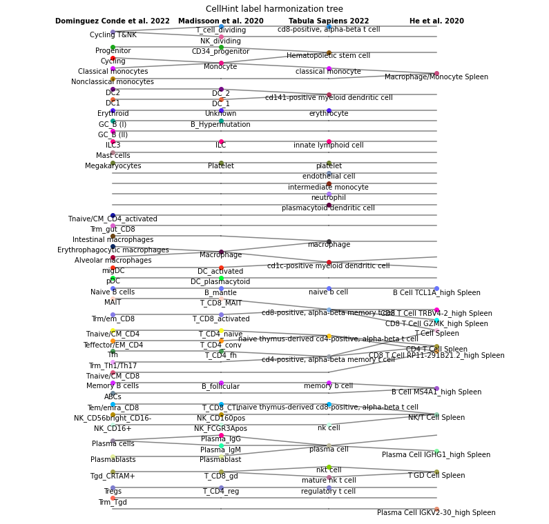
In a tree plot, each column is a dataset and cell types are connected across datasets. By default, cell types belonging to one low hierarchy (one row in the harmonisation table) are in the same color. You can change the color scheme by providing a data frame to the node_color parameter, with three consecutive columns representing dataset, cell type, and color (in hex code), respectively. node_color can also be a data frame with columns of dataset, cell type, and numeric value (for mapping color gradient in combination with cmap). Other parameters controlling the appearance of the tree plot (node shape, line width, label size, figure size, etc.) are detailed in cellhint.treeplot.

By changing the dataset (column) order in each high-hierarchy cell type, broader (more divisible) cell types can be positioned to the left, followed by fine-grained cell types to the right. The resulting plot shows how different authors group these cell types, thereby being more characteristic of the potential underlying biological hierarchy. This hierarchy can be generated and visualised by adding order_dataset = True.

cellhint.treeplot(alignment, order_dataset = True)

Because each high-hierarchy cell type is independent of each other, the new orders of datasets will be different across groups. To recognise the dataset origin of each cell type within the hierarchy, you can assign the same color or shape to cell types from the same dataset using the parameter node_color or node_shape.

cellhint.treeplot(alignment, order_dataset = True, node_shape = ['x', 'o', '^', '+'])

Alternatively, since only the harmonisation table (alignment.relation) is used when plotting this tree, cellhint.treeplot also accepts the input directly from the table. This is more convenient as a table is easier to manipulate, such as writing it out as a csv file and loading it later for tree plot.

# Write out the harmonisation table as a csv file.
# Note - if cell type names contain commas, set a different `sep` here.
alignment.relation.to_csv('cellhint_demo_folder/Spleen_HT.csv', sep = ',', index = False)

Read the harmonisation table and visualise top 20 rows.

import pandas as pd
HT = pd.read_csv('cellhint_demo_folder/Spleen_HT.csv', sep = ',')
cellhint.treeplot(HT.iloc[:20])

Visualise Group22.

cellhint.treeplot(alignment.relation[alignment.groups == 'Group22'])

In the tree plot, the order of datasets is the same with that in the harmonisation table (alignment.relation).

CellHint provides a method .best_align() to change the order of datasets post-harmonisation. Through this, datasets will be reharmonised in a different order (this post-harmonisation adjustment is more efficient than re-running cellhint.harmonize with a new order).

alignment.best_align(dataset_order = ['Tabula Sapiens 2022', 'He et al. 2020', 'Madissoon et al. 2020', 'Dominguez Conde et al. 2022'])

🖇 Harmonizing cell types of Tabula Sapiens 2022 and He et al. 2020
🖇 Harmonizing cell types of Madissoon et al. 2020
🖇 Harmonizing cell types of Dominguez Conde et al. 2022

A new harmonisation table will be generated in alignment.relation with the same dataset order as specified in .best_align.

alignment.relation.head(10)

	Tabula Sapiens 2022	relation	He et al. 2020	relation	Madissoon et al. 2020	relation	Dominguez Conde et al. 2022
0	endothelial cell	=	NONE	=	NONE	=	NONE
1	intermediate monocyte	=	NONE	=	NONE	=	NONE
2	neutrophil	=	NONE	=	NONE	=	NONE
0	NONE	=	NONE	=	NONE	=	ABCs
1	NONE	=	NONE	=	NONE	=	GC_B (II)
2	NONE	=	NONE	=	NONE	=	Tnaive/CM_CD4_activated
3	NONE	=	NONE	=	NONE	=	Trm_Tgd
4	NONE	=	NONE	=	NONE	=	Trm_gut_CD8
0	NONE	=	NONE	=	DC_plasmacytoid	=	pDC
1	UNRESOLVED	=	UNRESOLVED	=	B_Hypermutation	=	GC_B (I)

After changing the dataset order and reharmonising cell types, cells need to be reannotated based on the newly generated harmonisation table using the method reannotate.

alignment.reannotate()

Similarly, new information of reannotated cells is stored in alignment.reannotation.

Visualise this harmonisation result which now has a new dataset order.

cellhint.treeplot(alignment)

Importantly, as well as a full dataset list, you can provide a subset of datasets for reharmonisation in .best_align. This is useful in terms of focusing on part of the data.

alignment.best_align(dataset_order = ['Tabula Sapiens 2022', 'He et al. 2020'])

🖇 Harmonizing cell types of Tabula Sapiens 2022 and He et al. 2020

alignment.reannotate()

Note that after best_align and reannotate,new alignment.relation and alignment.reannotation will overwrite the old ones.

cellhint.treeplot(alignment)

Sankey plot

The other way to visualise harmonised cell types is the Sankey plot by cellhint.sankeyplot. CellHint builds this plot on the plotly package. plotly is not mandatory when installing CellHint, so you need to install it first if you want a visualisation form of Sankey diagram (and engines for exporting images such as kaleido).

import plotly.io as pio
pio.renderers.default = "iframe"

# Load previously saved harmonisation result and visualise it.
alignment = cellhint.DistanceAlignment.load('cellhint_demo_folder/spleen_alignment.pkl')
cellhint.sankeyplot(alignment)

This diagram shows how cell types are connected across datasets. Parameters controlling the appearance of the Sankey plot (node color, link color, figure size, etc.) are detailed in cellhint.sankeyplot.

Similar to the tree plot, since only the harmonisation table (alignment.relation) is used when plotting this Sankey diagram, cellhint.sankeyplot also accepts the input directly from the table. Thus you can manipulate this table and visualise it flexibly.

# Visualise top 30 rows for example.
cellhint.sankeyplot(alignment.relation.iloc[:30])

Export the plot if needed.

# Export the image as html.
cellhint.sankeyplot(alignment, show = False, save = 'cellhint_demo_folder/Spleen_sankey.html')
# Export the image as pdf.
cellhint.sankeyplot(alignment, show = False, save = 'cellhint_demo_folder/Spleen_sankey.pdf')